Dynamical Coring
Introduction
In Nagel et al., 2019 this method was described in detail. It was shown, that it significantly improves the markovianity of the resulting microstates. It is a dynamical boarder correction methods which counts transitions only if they reach the dynamical core, remain longer than \(\tau_\text{cor}\) in it.
Execution
clustering noise -s state_file
                 -w window_file
                 -o output
                 -d Wi_output
                 --cores output_cores
                 --concat-nframes NFRAMES
                 --concat-limits limit_file
                 --iterative
                 -v
Parameters
Input Parameters
| Parameter | Description |
|---|---|
| \(\mathtt{\mbox{-}s :}\) | The name(path) of the clusterd state trajectory file. |
| \(\mathtt{\mbox{-}w :}\) | Either an integer which is interpreted as the same window for
all states, or The name(path) to the window size file. The file
should be formatted as a two-column file assigning to each
state a coring time \(\tau_\text{cor}\):
STATE_ID TAU_COR use * as STATE_ID to match all (other) states. e.g.:
\({}^*\ 20\) |
| \(\mathtt{\mbox{--}concat\mbox{-}nframes:}\) | The number of frames per (equally sized) sub-trajectories for concatenated trajectory files. |
| \(\mathtt{\mbox{--}concat\mbox{-}limits:}\) | The name(path) to the limit file. It should be a single column file with the length of each trajectory. for a concatenated trajectory of three chunks of sizes 100, 50 and 300 frames: '100 50 300'. |
Output Parameters
| Parameter | Description |
|---|---|
| \(\mathtt{\mbox{-}o}\) | Filename for the output file of the noise corrected microstates. |
| \(\mathtt{\mbox{-}d}\) | Basename for the probability distributions \(W_i(t)\). |
| \(\mathtt{\mbox{--}cores}\) | Filename where the microstate trajectory is stored with all frames which are not in the core regions denoted by \(-1\). |
Miscellaneous Parameters
| Parameter | Description |
|---|---|
| \(\mathtt{\mbox{-}\mbox{-}iterative}\) | Increase coring time frame by frame until specified window. |
| \(\mathtt{\mbox{-}v}\) | Verbose mode with some output. |
Detailed Description
Transitions between states usually do not occur in a direct and discrete manner. Rather, the system goes into a 'transition zone', where frames are alternating fast between two states before staying in the new state. These alternations severely change the dynamical description of the system and produce artificially short life times. You can use variable dynamic coring to correct for these boundary artifacts. Here, 'dynamic' means that we refer to the core of a state, if the system stays inside for a given amount of time (the so-called coring time). Thus, we check dynamic properties instead of geometric ones.
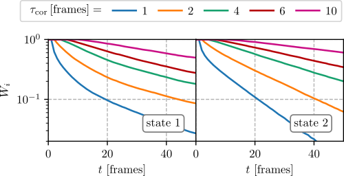
To identify the optimal coring time \(\tau_\text{cor}\), run the coring-algorithm for several coring times and plot the probability \(W_i(t)\) to stay in state \(i\) for duration \(t\) (without considering back transitions). The optimal coring time is the lowest that matches an exponential decay. To produce probability distribution for different coring times, write a \(\mathtt{win}\) file with the content
* CORING_TIME
where \(\mathtt{CORING\_TIME}\) is the croing time given as number of frames. The star means, that we treat all states with the same coring time. Starting from v1.2 one can also pass the integer directly to the function call with \(\mathtt{\mbox{-}w\ CORING\_TIME}\). Even though, the coring time can be specified separatly for all states, it is recommended to take a common time. Then run the command with the \(\mathtt{\mbox{-}d}\) flag and without the \(\mathtt{\mbox{-}o}\).
This produces several files of the format \(\mathtt{Wi\_CORING\_TIME}\). Repeat this process several times for different choices of coring time in the \(\mathtt{win}\) file.
After the generation of the probability \(W_i(t)\) files, plot them (e.g. with matplotlib) and select the window size that shows an exponential decay. In most cases it is sufficient to take the same window for all states. Select the window such that it shows an exponential decay for all microstates. In the following figures the probabilities for the first two states are shown,

where see that \(\tau_{cor}=4\,[\text{frames}]\) is sufficient.
When you have selected proper windows sizes for all states, rewrite your \(\mathtt{win}\) file to reflect these. For three different states \(1, 2\,\&\,3\), e.g. you could write
  1 100
  2 200
  3 75
for window sizes of 100 frames for state 1, 200 frames for state 2 and 75 frames for state 3.
Finally, to produce the cored cluster trajectory, run the command with the \(\mathtt{\mbox{-}o}\) flag and without the \(\mathtt{\mbox{-}d}\) flag.