Building a Network
Introduction
In this step a network representation of the previously obtained clusters is build. This enables us to find the local minima of the free energy landscape.
Execution
clustering network -p minimal_population
                   -o output_basename
                   -b basename
                   --min fe_min
                   --step fe_step
                   --max fe_max
                   --network-html
                   -v
Parameters
Input Parameters
| Parameter | Description |
|---|---|
| \(\mathtt{\mbox{-}p :}\) | Minimal population defines the critical population limit that a cluster can form a seed. Default is \(1\). |
| \(\mathtt{\mbox{-}b :}\) | Specify the basename of cluster output files. In general it is the previously used option of output.(see previous step \(\mathtt{\mbox{-}o}\)). Default: \(\mathtt{clust}\). |
| \(\mathtt{\mbox{--}min :}\) | Specify from which free energy it starts (see previous step \(\mathtt{\mbox{-}T}\)). Default: \(0.10\). |
| \(\mathtt{\mbox{--}step :}\) | Specify the step width in which the free energy is scanned (see previous step \(\mathtt{\mbox{-}T}\)). Default: \(0.00\), which corresponds to highest free energy. |
| \(\mathtt{\mbox{--}max :}\) | Specify the final free energy it should scan (see previous step \(\mathtt{\mbox{-}T}\)). Default: \(0.10\). |
Output Parameters
| Parameter | Description |
|---|---|
| \(\mathtt{\mbox{-}o}\) | Basename for the output files. Default: \(\mathtt{network}\). radius. |
Miscellaneous Parameters
| Parameter | Description |
|---|---|
| \(\mathtt{\mbox{--}network\mbox{-}html}\) | If this flag is set, a html representation of the network will be generated. For many states (low value of \(\mathtt{\mbox{-}p}\) this may take long. |
| \(\mathtt{\mbox{-}v}\) | Verbose mode with some output. |
Detailed Description
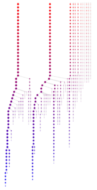
The net result of the screening process is a list of files (here: \(\mathtt{cluster.^*}\)) defining the cluster membership per frame for different free energy thresholds. Using these memberships, we can derive a network of microstates that reflects their respective geometrical similarity. The network has a (multi-)tree structure, with nodes defining separate microstates at the various free energy levels. In case two (or more) clusters grow big enough to be geometrically close, they will be merged into a single node at the free energy level, at which they are not distinguishable from a single state.
If the metastable states of the free energy landscape are geometrically diverse enough, the network will form several trees in parallel, without them being joined at the highest free energy level. Of course, you can add a virtual root node at a free energy level above the maximum to join all trees into a single tree, however this has to be done manually. The clustering program will not artificially join the separate trees.
This is the first step to get states out of the clusters. The idea is to identify local minima in the free energy landscape. Here we scan again through the free energy landscape. A cluster is accepted as node if it:
- is geometrically disconnected to all accepted clusters (nodes)
- is not at highest free energy
- has a population higher than the minimal population \(P_\text{min}\)
The concept of minimal population should be used carefully. It should only be used to remove local fluctuation within a minimum and not to lump close minima. Latter is non physical and leads to bad defined states. If one is interested in macrostates a dynamical clustering method, e.g. MPP, should be used.
Once we have the clusters we need to generate states. The first step is to identify the local minima of the free energy landscape. This is achieved by running
clustering network -p 500 --network-html --basename cluster -v
The minimal population \(\mathtt{\mbox{-}p}\) should be selected high enough to guarantee that all local fluctuations are ignored, but no minima.
This command generates many output files. For the sake of readability we assume that the output basename was set to the default value. In the following we will discuss them briefly:
- \(\mathtt{remapped\_basename.*}\): These are essentially identical to the input files (\(\mathtt{basename.*}\), but differ in an important aspect: every id at a high(er) free energy level, that has already been assigned to a microstate at a lower level will be given a new, unique id to distinguish the states at every free energy level from each other. This is necessary, since the various input files define microstates only locally, at their respective free energy level - and all of them use the same range of integers (\(1 \ldots N\)) as ids.
- \(\mathtt{network\_nodes.dat}\): The different nodes of the network, representing the microstates at different free energy levels. The file contains all nodes with id, free energy level and population.
- \(\mathtt{network\_links.dat}\): The links connecting the network nodes. This file holds the information which microstates will be lumped together at higher free energy levels.
- \(\mathtt{network\_leaves.dat}\): All network leaves, i.e. nodes (microstates) without child nodes at a lower free energy level. These microstates represent the minima of their local basins.
- \(\mathtt{network\_end\_node\_traj.dat}\): A clustered trajectory, in which all frames belonging to the end nodes (or leaves) are marked by their respective microstate id. All frames, that do not belong to a leaf, will be marked as zero. This trajectory will act as a seed for the complete separation of the free energy landscape into different microstates, assigning every single frame to a suitable state.
- \(\mathtt{network\_visualization.html}\): This file is only generate if \(\mathtt{\mbox{--}network\mbox{-}html}\) flag is used. Open this file with a modern web browser to get a simple representation of the generated network. An example is shown in the following figure. Rendering will only work in reasonable time, if the number of microstates is not too high. You can control this with the \(\mathtt{\mbox{-}p}\) option. Controls: Single left click on a node for detailed information. Press and hold left on empty area until cursor is marked by a circle to drag the network. Use mouse wheel to zoom in and out.