Clustering Documentation - a code documentation for the clustering package

Introduction

This tutorial explains how to use the clustering program provided at github.com/moldyn/clustering . A general introduction to the idea of dimensionality reduction and clustering can be found in Sittel et al., 2018.

The density-based clustering algorithm used in the module $\mathtt{density}$ consists of four parts:

Calculate the free energy for each point based on the local point density.
Scan the free energy landscape (from minimal to maximal value) and assign all points into geometrical clusters. If a point $i$ is geometrically close to an existing cluster ($d_{ij}\lt d_\text{lump}$), it is assigned to it. Otherwise it forms a new cluster.
Scan another time through the free energy to identify the seeds of microstates.
The microstates are formed by assigning every point that is not yet part of a seed to its geometrically closest neighbor with lower energy. This guarantees that the barriers are cut at the edges.

Each of these steps will be discussed in detail in the following. Afterwards we discuss two methods which improve the microstate definitions on the barriers, namely $\mathtt{noise}$ and $\mathtt{coring}$. Further, we present the most probable path algorithm ($\mathtt{mpp}$) to dynamically lump the microstates into macrostates.

Preparing the data

Apply a suitable dimension reduction method (e.g. PCA) on the data and select a limited number of essential coordinates. For more information on PCA see FastPCA. It is important not to exceed the maximum dimensionality for the given sampling when using a density-based clustering approach. Too high dimensionality will suffer from the 'Curse of Dimensionality'. A good estimate, e.g. for a six dimensional data set is a sampling of $\gt 10^6$ frames.

The input data for the clustering package needs to be column-oriented, space-separated plain text. It is possible to use concatenated trajectory files.

From now on, let's assume we have prepared input data for clustering in the file $\mathtt{coords}$. Further, we assume that it is a single trajectory. Otherwise, the $\mathtt{\mbox{-}\mbox{-}concat\mbox{-}limits}$ or $\mathtt{\mbox{-}\mbox{-}concat\mbox{-}nframes}$ needs to be used in the steps $\mathtt{noise}$ and $\mathtt{coring}$. If you do not yet have suitable data, you download the example data set. Download the data, e.g., with $\mathtt{wget}$, unpack it with $\mathtt{bzip2}$ and create a symlink called $\mathtt{coords}$ to be in line with the rest of the tutorial:

     
       wget http://www.moldyn.uni-freiburg.de/software/aib9.pca.reduced.bz2

       bunzip2 aib9.pca.reduced.bz2

       ln -s aib9.pca.reduced coords

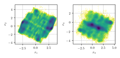
If your computer is missing any of these programs, install them (or let the sysadmin do it). If they are not available, you are probably not able to install the package. The data consists of $\sim 1.4 \cdot 10^6$ frames of a simulation of the peptide Aib9 (for more information on this data set, see Buchenberg et al., 2015), reduced to four essential coordinates based on a principal component analysis using dihedral angles. The following figure shows the 2D projections along principal components $x_1, x_2$ and $x_3,x_4$ to give an impression of the free energy landscape.

Calculating the free energy and nearest neighbors

Other than k-means, this density-based clustering algorithms estimates the optimal seeds of the microstates. Those are regions with local high density representing local minima in the free energy landscape. Latter is calculated with $$ G_{R}(\vec{r})= - \ln (P_R(\vec{r})/P_{R}^{\text{max}}), $$ where $P_{R}(\vec{r})$ is the local population at the point $\vec{r}$ with respect to the sphere of radius $R$.

The coordinate file named $\mathtt{coords}$ is the only needed input for generating the free energy/ population and nearest neighbor files. This can be done simply by running:

             
             clustering density -f coords -p pop -d fe -b nn -v

In Nagel et al., 2019 it was shown that in most cases the lumping radius $d_\text{lump}$ is a good choice for the clustering radius $R$. Hence, we do not use the flag $\mathtt{\mbox{-}r}$ here to set $R = d_\text{lump}$. Nonetheless, in some cases (eg. if the sampling is relatively high and the dimensionality rather small) $R$ should be chosen differently. It should be noted, that $R$ and $d_\text{lump}$ are in general independet variabels: while $R$ needs to be small enough to ensure local constant density, $d_\text{lump}$ determines only the desired level of coarse-graining.

This code generates the population file $\mathtt{pop}$, the free energy file $\mathtt{fe}$ and the four column nearest neighbor file $\mathtt{nn}$. This step is here only for pedagogical reasons. If we replace in the next step $\mathtt{\mbox{-}D}$/$\mathtt{\mbox{-}B}$ with $\mathtt{\mbox{-}d}$/$\mathtt{\mbox{-}b}$ we can achieve both steps within one.

Energy Screening - Generating Clusters

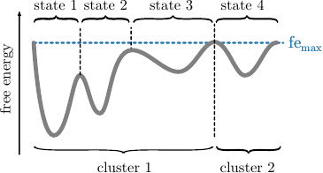
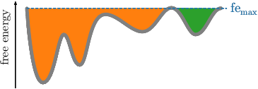
Before we explain the procedure, we want to note here that clusters do not correspond to states. Clusters just separate the space into geometrically connected regions. Those are per construction separated at the highest (considered) free energy, while states are separated at all barriers. At the highest free energy, when all trajectory points are considered, the main cluster usually contains up to $90\%$ of all frames. This is illustrated in the following figure.

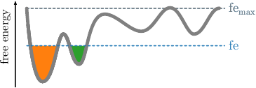
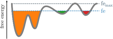
Given the readily computed free energies ($\mathtt{\mbox{-}d}$) and neighborhoods ($\mathtt{\mbox{-}b}$) per frame for the selected radius, we continue the clustering by screening the free energy landscape. This means, we choose a (initially low) free energy cutoff $\tilde{G}$ and select all frames below. They are combined into clusters, if they are geometrically connected with respect to the lumping distance $d_\text{lump}=2\sigma$. The latter is automatically computed from the MD data. $\sigma$ denotes here the standard deviation of the nearest neighbor distances. An illustration is provided in the following figures. If the threshold raises, previous clusters can be merged.

This is done repeatedly, with increasing free energy cutoffs. The end result will be multiple plain-text files, one for each cutoff, that define cluster trajectories. Their format is a single column of integers, which act as a membership id of the given frame (identified by the row number) to a certain cluster. For each file, the microstate ids start with the value 1 and are numbered incrementally. All frames above the given free energy threshold are denoted by $0$, which acts as a kind of melting pot for frames with unknown affiliation.

Do not worry if there are still frames denoted by $0$ in the cluster file of the highest free energy. The clustering program rounds the maximum free energy to 2 decimal places for screening, which may result in a cutoff that is slightly lower than the true maximum. Thus, there may be frames left, which are not assigned to a cluster since they are not below the cutoff.

However, since we are going to generate states from selecting the basins of the clusters and 'filling up' the free energy landscape from bottom to top, these states are not interesting on their own, anyhow, and will be assigned to a distinct state in the next step.

The coordinate file named $\mathtt{coords}$, the previous generated free energy ($\mathtt{fe}$) and nearest neighbors ($\mathtt{nn}$) files are all needed for generating the clusters. This can be done simply by running:

             
                clustering density -f coords -T -1 -D fe -B nn -o cluster -v

With $\mathtt{\mbox{-}T\ \mbox{-}1}$ the default screening step width of $0.1$ is selected and $\mathtt{\mbox{-}o\ cluster}$ sets the basename of the generated output files. If you do not have calculated the free energy file and the nearest neighbor yet, just substitute $\mathtt{\mbox{-}D}$/$\mathtt{\mbox{-}B}$ with $\mathtt{\mbox{-}d}$/$\mathtt{\mbox{-}b}$. In this step clusters (geometrically connected regions) are generated for all points below the free energy threshold, e.g., for $\mathtt{cluster.2.6}$ all points with free energy $\Delta G \le 2.6\, \text{k}T$ are used. The files are single column files.

Building a network

The net result of the screening process is a list of files (here: $\mathtt{cluster.^*}$) defining the cluster membership per frame for different free energy thresholds. Using these memberships, we can derive a network of microstates that reflects their respective geometrical similarity. The network has a (multi-)tree structure, with nodes defining separate microstates at the various free energy levels. In case two (or more) clusters grow big enough to be geometrically close, they will be merged into a single node at the free energy level, at which they are not distinguishable from a single state.

If the metastable states of the free energy landscape are geometrically diverse enough, the network will form several trees in parallel, without them being joined at the highest free energy level. Of course, you can add a virtual root node at a free energy level above the maximum to join all trees into a single tree, however this has to be done manually. The clustering program will not artificially join the separate trees.

This is the first step to get states out of the clusters. The idea is to identify local minima in the free energy landscape. Here we scan again through the free energy landscape. A cluster is accepted as node if it:

is geometrically disconnected to all accepted clusters (nodes)
is not at highest free energy
has a population higher than the minimal population $P_\text{min}$

The concept of minimal population $P_\text{min}$ should be used carefully. It should only be used to remove local fluctuation within a minimum and not to lump close minima. Latter is non-physical and leads to bad defined states. If one is interested in macrostates a dynamical clustering method, e.g. MPP, should be used. In the following figures we compare the number of resulting states $k$ with the minimal population $P_\text{min}$. To be comparable between different data sets, $P_\text{min}$ is usually given in percent of the total number of frames. For obtaining this plot we used $\mathtt{noise}$ with $c_\text{min}=0.1$.

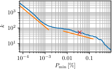
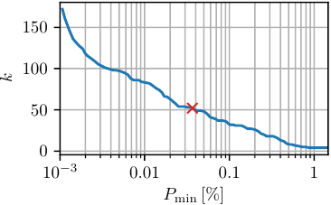
One should always choose an $P_\text{min}$ value large enough to avoid the initial drop (shown in the first figure). Depending on the desired coarse-graining, one can pick a value in the range of $P_\text{min}\in[4\cdot10^{-4}-0.2]$. In the following we take $P_\text{min}=500$

Once we have the clusters, we need to generate states. The first step is to identify the local minima of the free energy landscape. This is achieved by running

             
              clustering network -p 500 --network-html --basename cluster -v

The minimal population $\mathtt{\mbox{-}p}$ should be selected high enough to guarantee that all local fluctuations are ignored, but no minima.

Generate a microstate trajectory

By defining the clustered trajectory of basin centers, we seed the clustering process with a limited number of microstates. The clustering program will use this information to assign all unassigned frames to one of these microstates. This is done by 'filling' the basins, i.e. starting at the unassigned frame of the lowest free energy, it will identify the closest microstate and add the given frame to its population. With the updated clustering trajectory, this process is repeated until no frame is left unassigned.

To separate the tree at its 'leaf-branches', i.e., to assign all frames in the trajectory to a distinct microstate, run

             
  clustering density -f coords -i network_end_node_traj.dat -D fe -B nn -o microstates -v

The end result of the geometric, density-based clustering is the $\mathtt{microstates}$ file, which holds a single column with microstate id / frame, where the row number equals the according frame number. The resulting microstates ids are ordered by their population.

To get a first idea about the microstates one can simply run

             
  clustering stats -s microstates

This returns the population of each state. Further, for all states the number of entering is stated. This number should be much smaller than the population, otherwise this indicates a short metastability.

Noise correction

On the barriers we are facing a poor sampling. Therefore, also due to projection artefacts, frames can be assigned to the wrong state. To avoid this, we simply reassign those frames dynamically instead of geometrically. This was proposed in Nagel et al., 2019. We use the following definition of noise:

All geometrically isolated clusters with population lower than $\mathtt{c_\text{min}}$ are assigned as noise.
They are assigned dynamically (in the sense of coring) to the previously visited state.

Where $\mathtt{c_\text{min}}$ is given in percent of the total population. This has an impact of

$\approx5\%$ of total frames
improves the Markovianity in some systems

This all can be achieved by running

             
clustering noise -s microstates -c 0.1 -o microstatesNoise --basename cluster -v

The result is the $\mathtt{microstatesNoise}$ file, which holds a single column with microstate id / frame, where the row number equals the according frame number.

Remember that if you are using a concatinated trajectory you need to specify the limits by passing either $\mathtt{\mbox{-}\mbox{-}concat\mbox{-}limits}$ or $\mathtt{\mbox{-}\mbox{-}concat\mbox{-}nframes}$.

Dynamical coring

Transitions between states usually do not occur in a direct and discrete manner. Rather, the system goes into a 'transition zone', where frames are alternating fast between two states before staying in the new state. These alternations severely change the dynamical description of the system and produce artificially short life times. You can use variable dynamic coring to correct for these boundary artifacts. Here, 'dynamic' means that we refer to the core of a state, if the system stays inside for a given amount of time (the so-called coring time). Thus, we check dynamic properties instead of geometric ones.

To identify the optimal coring time $\tau_\text{cor}$, run the coring-algorithm for several coring times and plot the probability $W_i(t)$ to stay in state $i$ for duration $t$ (without considering back transitions). The optimal coring time is the lowest that matches an exponential decay. To produce probability distribution for different coring times, write a $\mathtt{win}$ file with the content

             
  * CORING_TIME

where $\mathtt{CORING\_TIME}$ is the coring time given as number of frames. The star means, that we treat all states with the same coring time. Even though, the coring time can be specified separatly for all states, it is recommended to take a common time. Then run the command

             
  clustering coring -s microstatesNoise -w win -d Wi -v

This produces several files of the format $\mathtt{Wi\_CORING\_TIME}$. Repeat this process several times for different choices of coring time in the $\mathtt{win}$ file.

Remember that if you are using a concatinated trajectory you need to specify the limits by passing either $\mathtt{\mbox{-}\mbox{-}concat\mbox{-}limits}$ or $\mathtt{\mbox{-}\mbox{-}concat\mbox{-}nframes}$.

After the generation of the probability $W_i(t)$ files, we plot them (e.g. with matplotlib) and select the smallest window size that shows an exponential decay. In most cases it is sufficient to take the same window for all states. Select the window such that it shows an exponential decay for all microstates. In the following figures the probabilities for the first two states are shown,

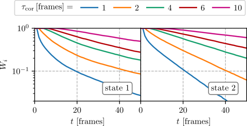
where we see that $\tau_{cor}=4\,\text{frames}$ is sufficient.

When you have selected proper windows sizes for all states, rewrite your $\mathtt{win}$ file to reflect these. For three different states $1, 2\,\&\,3$, e.g. you could write

for window sizes of 100 frames for state 1, 200 frames for state 2 and 75 frames for state 3.

Finally, to produce the cored cluster trajectory, run

             
  clustering coring -s microstatesNoise -w win -o microstatesFinal -v

If one wants to understand the effect of coring better, as a first step one can take a look at the different statistics by running

             
  clustering stats -s microstatesFinal

as well as for the uncored trajectory ($\mathtt{microstates}$) This reveals that the metastability highly improves due to coring. It should be noted that if one wants to geometrically interpreted the final states one can use the $\mathtt{filter}$ module. Therewith, one can get all frames of the input coordinates belonging to a certain state. This module is also capable of splitting xtc (gromacs) trajectories. Hence, if one uses the backbone dihedral angles to cluster, one can easily split also the MD trajectory to further investigate the states.

For a geometrical interpretation of the states one can also use the ramacolor script which was introduced in Sittel et al., 2016.

Dynamical clustering - MPP

This method was proposed in Jain et al., 2014. To get a dynamical description of the state space, use the $\mathtt{MPP}$ method to cluster the geometric microstates by their respective transition probabilities. This way, we identify the dynamically more stable from the less stable states. The most important parameter for MPP is the lagtime $\tau_\text{mpp}$, which is - for the clustering program - always given in numbers of frames. The lagtime in units of time is trivially given by its value in numbers of frames multiplied by the time step of the underlying simulation.

The lagtime is the amount of time (or number of frames) that is skipped when calculating transition probabilities from one state to another. In effect, timescales below the given lagtime are discarded and the dynamical clustering will only be able to describe processes of length higher than the given lagtime. It acts as a control parameter to blend out (uninteresting) processes on too short timescales and focus on processes of essential motion, which typically happen at longer timescales as the simulation stepping.

Additionally, at a high enough lagtime the system will be approximately markovian, resulting in a discrete set of states well described by markovian dynamics.

To run MPP, use the command

             
  clustering mpp -s microstatesFinal -D fe -l 25 -v

where $\mathtt{\mbox{-}l}$ is the lagtime in units of frames.

The MPP run generates lots of new files, per default called $\mathtt{mpp\_pop\_^*}$ and $\mathtt{mpp\_traj\_^*}$. The star stands for the metastability ($Q_\text{min}$-value) of the run. The $\mathtt{{}^*pop^*}$-files hold the population information of the clusters for the given metastibility, while the $\mathtt{{}^*traj^*}$-files are the resulting cluster trajectories.

The metastability value controls, how stable a state has to be to remain as single state. All states with a stability less then the given $Q_\text{min}$-value will be lumped according to their most probable state-path.

Let's assume from now on that the clustering resolution of choice is given at a metastability of 0.80. Thus, the clustered trajectory is in the file $\mathtt{mpp\_traj\_0.80}$.

Tutorial